Changelog

New updates and improvements at Cloudflare.

Jul 8, 2026

Query R2 Data Catalog tables with R2 SQL from the dashboard

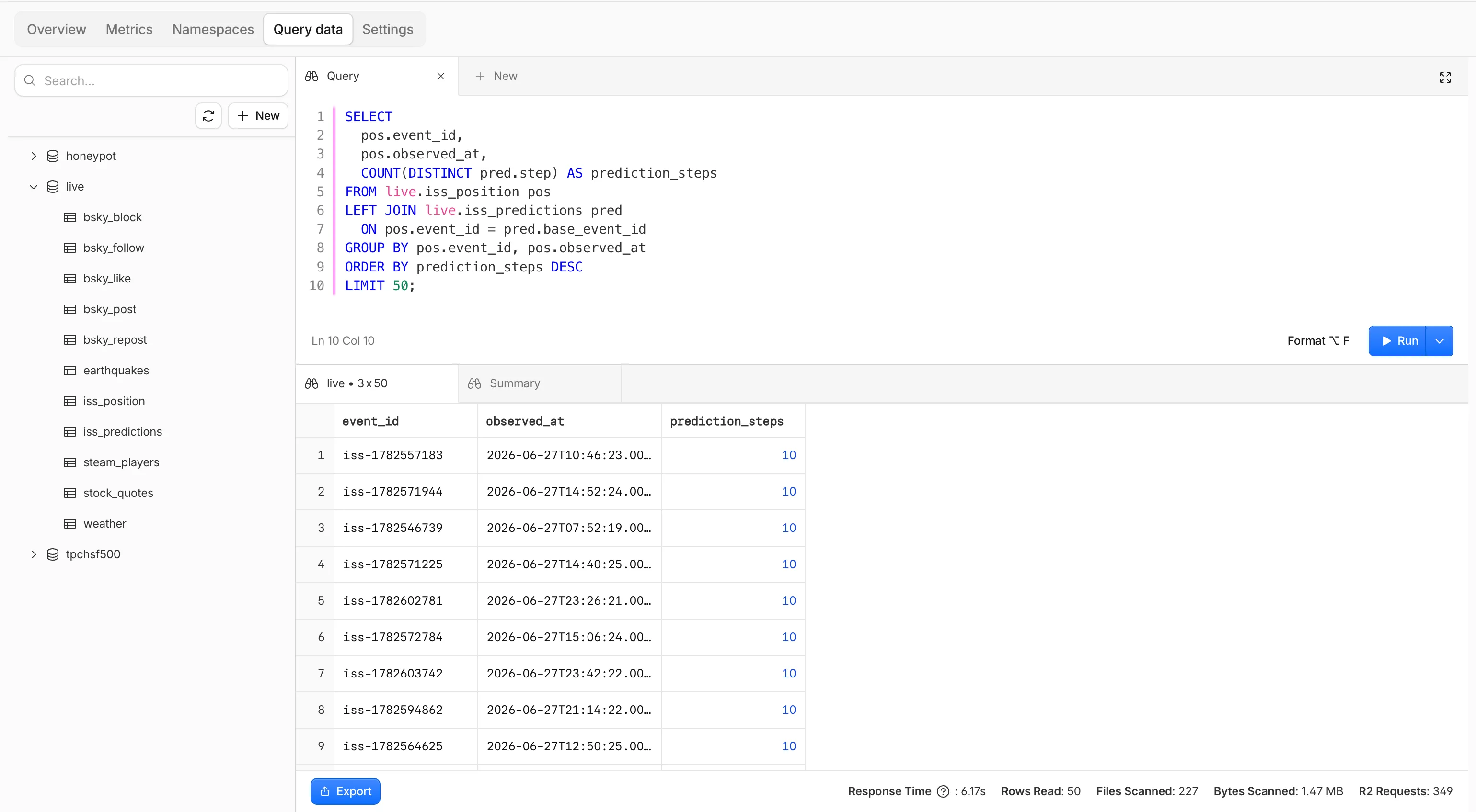
You can now query your R2 Data Catalog tables with R2 SQL directly from the Cloudflare dashboard, without installing a CLI or wiring up a client. This makes it easy to explore your Apache Iceberg ↗ data, validate queries, and inspect results in one place.

To get started, go to R2 Data Catalog ↗ in the Cloudflare dashboard and select Query data to launch the built-in SQL editor. From there you can:

Write and run queries interactively — Iterate on R2 SQL directly in the browser with syntax highlighting and autocomplete, instead of re-running commands through Wrangler or the REST API.
Explore your data — Explore your namespaces and tables alongside the editor so you can discover what's queryable without leaving the page or using other tools.
Understand results and performance — View result sets with per-query statistics, export them, and get helpful EXPLAIN outputs to see exactly how a query runs.

Jun 22, 2026

R2 SQL now supports window functions, DISTINCT, and set operations

R2 SQL

R2 SQL now supports window functions, SELECT DISTINCT, set operations, and additional aggregates, making it easier to write analytical queries without preprocessing your data elsewhere.

R2 SQL is Cloudflare's serverless, distributed SQL engine for querying Apache Iceberg ↗ tables stored in R2 Data Catalog.

New capabilities

Window functions — ROW_NUMBER, RANK, DENSE_RANK, PERCENT_RANK, CUME_DIST, NTILE, LAG, LEAD, FIRST_VALUE, LAST_VALUE, NTH_VALUE, and aggregates with an OVER (...) clause, including PARTITION BY and explicit frames
QUALIFY — filter rows based on a window function result
DISTINCT — SELECT DISTINCT, DISTINCT ON (...), and the DISTINCT modifier on aggregates such as COUNT(DISTINCT ...)
Set operations — UNION, UNION ALL, INTERSECT, and EXCEPT
Grouping extensions — GROUPING SETS, ROLLUP, and CUBE
Exact aggregates — MEDIAN, PERCENTILE_CONT, ARRAY_AGG, and STRING_AGG

Examples

Rank rows with a window function

SELECT customer_id, region,
       ROW_NUMBER() OVER (PARTITION BY region ORDER BY total_amount DESC) AS rank_in_region
FROM my_namespace.sales_data

Filter with QUALIFY

SELECT customer_id, region, total_amount
FROM my_namespace.sales_data
QUALIFY ROW_NUMBER() OVER (PARTITION BY region ORDER BY total_amount DESC) <= 3

Combine tables with a set operation

SELECT customer_id FROM my_namespace.sales_data
EXCEPT
SELECT customer_id FROM my_namespace.archived_sales

The named WINDOW clause is not supported — inline the OVER (...) specification at each call site. For the full syntax reference, refer to the SQL reference. For supported features and performance guidance, refer to Limitations and best practices.

Jun 8, 2026

R2 SQL now supports UNION, INTERSECT, EXCEPT, and SELECT DISTINCT

R2 SQL

R2 SQL now supports set operations (UNION, INTERSECT, EXCEPT) and SELECT DISTINCT, expanding the range of analytical queries you can run directly on Apache Iceberg ↗ tables in R2 Data Catalog.

Set operations

Combine the results of multiple SELECT statements:

UNION — returns all rows from both queries, removing duplicates
UNION ALL — returns all rows from both queries, including duplicates
INTERSECT — returns only rows that appear in both queries
EXCEPT — returns rows from the first query that do not appear in the second

-- Find zones that had either firewall blocks OR high-risk requests
SELECT zone_id FROM my_namespace.firewall_events WHERE action = 'block'
UNION
SELECT zone_id FROM my_namespace.http_requests WHERE risk_score > 0.8

-- Find zones with both firewall blocks AND high traffic
SELECT zone_id FROM my_namespace.firewall_events WHERE action = 'block'
INTERSECT
SELECT zone_id FROM my_namespace.http_requests
GROUP BY zone_id
HAVING COUNT(*) > 10000

-- Find enterprise zones that have not been compacted
SELECT zone_id FROM my_namespace.zones WHERE plan = 'enterprise'
EXCEPT
SELECT zone_id FROM my_namespace.compaction_history

Select distinct

Eliminate duplicate rows from query results:

SELECT DISTINCT region, department
FROM my_namespace.sales_data
WHERE total_amount > 1000
ORDER BY region, department
LIMIT 100

For large datasets where approximate results are acceptable, approx_distinct() remains a faster alternative for counting unique values.

For the full syntax reference, refer to the SQL reference. For performance guidance, refer to Limitations and best practices.

May 28, 2026

R2 SQL pricing announced

R2 SQL

R2 SQL is a serverless, distributed query engine that runs SQL against Apache Iceberg ↗ tables stored in R2 Data Catalog. R2 SQL now has published pricing based on a single dimension: the volume of compressed data scanned to execute your queries. At $2.50 / TB ($ 0.0025 / GB), R2 SQL is priced at half the cost of AWS Athena and less than half of Google BigQuery on-demand.

Billing is not yet enabled. We will provide at least 30 days notice before we start charging for R2 SQL usage.

Data scanned is measured on compressed bytes read from R2 object storage. This matches what you see in your R2 bucket — if a Parquet file is 100 MB on disk, scanning that file bills for 100 MB. Each query has a minimum billing increment of 10 MB.

Free plans include 1 GB / month and Paid plans include 10 GB / month. Standard R2 storage and operations and R2 Data Catalog charges apply separately.

For full pricing details and billing examples, refer to R2 SQL pricing.

May 15, 2026

R2 SQL now supports JOINs, subqueries, and multi-table queries

R2 SQL

R2 SQL is Cloudflare's serverless, distributed SQL engine for querying Apache Iceberg ↗ tables stored in R2 Data Catalog. R2 SQL runs directly on Cloudflare's global network with no infrastructure to manage, so you can analyze data in R2 without exporting it to an external warehouse.

R2 SQL now supports joining multiple Iceberg tables in a single query. You can combine tables with JOINs, filter with subqueries, and define multi-table CTEs to build complex analytical queries.

New capabilities

JOINs — INNER JOIN, LEFT JOIN, RIGHT JOIN, FULL OUTER JOIN, CROSS JOIN, and implicit joins (comma-separated FROM with conditions in WHERE)
Subqueries — IN / NOT IN, EXISTS / NOT EXISTS, scalar subqueries in SELECT / WHERE / HAVING, and derived tables (subqueries in FROM)
Multi-table CTEs — WITH clauses can reference different tables and include JOINs
Self-joins — join a table with itself using different aliases
Multi-way joins — join three or more tables in a single query

Examples

Two-table JOIN with aggregation

SELECT z.domain, z.plan, COUNT(*) AS request_count
FROM my_namespace.zones z
INNER JOIN my_namespace.http_requests h ON z.zone_id = h.zone_id
WHERE z.plan = 'enterprise'
GROUP BY z.domain, z.plan
ORDER BY request_count DESC
LIMIT 20

`EXISTS` subquery

SELECT z.domain, z.plan
FROM my_namespace.zones z
WHERE EXISTS (
    SELECT 1 FROM my_namespace.firewall_events f
    WHERE f.zone_id = z.zone_id AND f.action = 'block'
)
ORDER BY z.domain
LIMIT 20

Multi-table CTE with JOIN

WITH top_zones AS (
    SELECT zone_id, COUNT(*) AS req_count
    FROM my_namespace.http_requests
    GROUP BY zone_id
    ORDER BY req_count DESC
    LIMIT 50
),
zone_threats AS (
    SELECT zone_id, COUNT(*) AS threat_count
    FROM my_namespace.firewall_events
    WHERE risk_score > 0.5
    GROUP BY zone_id
)
SELECT tz.zone_id, tz.req_count, COALESCE(zt.threat_count, 0) AS threat_count
FROM top_zones tz
LEFT JOIN zone_threats zt ON tz.zone_id = zt.zone_id
ORDER BY tz.req_count DESC
LIMIT 20

For the full syntax reference, refer to the SQL reference. For performance guidance with joins, refer to Limitations and best practices.

Apr 20, 2026

R2 SQL adds JSON functions, EXPLAIN FORMAT JSON, and unpartitioned table support

R2 SQL

R2 SQL is Cloudflare's serverless, distributed, analytics query engine for querying Apache Iceberg ↗ tables stored in R2 Data Catalog.

R2 SQL now supports functions for querying JSON data stored in Apache Iceberg tables, an easier way to parse query plans with EXPLAIN FORMAT JSON, and querying tables without partition keys stored in R2 Data Catalog.

JSON functions extract and manipulate JSON values directly in SQL without client-side processing:

SELECT
  json_get_str(doc, 'name') AS name,
  json_get_int(doc, 'user', 'profile', 'level') AS level,
  json_get_bool(doc, 'active') AS is_active
FROM my_namespace.sales_data
WHERE json_contains(doc, 'email')

For a full list of available functions, refer to JSON functions.

EXPLAIN FORMAT JSON returns query execution plans as structured JSON for programmatic analysis and observability integrations:

npx wrangler r2 sql query "${WAREHOUSE}" "EXPLAIN FORMAT JSON SELECT * FROM logpush.requests LIMIT 10;"

┌──────────────────────────────────────┐
│ plan                                 │
├──────────────────────────────────────┤
│ {                                    │
│   "name": "CoalescePartitionsExec",  │
│   "output_partitions": 1,            │
│   "rows": 10,                        │
│   "size_approx": "310B",             │
│   "children": [                      │
│     {                                │
│       "name": "DataSourceExec",      │
│       "output_partitions": 4,        │
│       "rows": 28951,                 │
│       "size_approx": "900.0KB",      │
│       "table": "logpush.requests",   │
│       "files": 7,                    │
│       "bytes": 900019,               │
│       "projection": [                │
│         "__ingest_ts",               │
│         "CPUTimeMs",                 │
│         "DispatchNamespace",         │
│         "Entrypoint",                │
│         "Event",                     │
│         "EventTimestampMs",          │
│         "EventType",                 │
│         "Exceptions",                │
│         "Logs",                      │
│         "Outcome",                   │
│         "ScriptName",                │
│         "ScriptTags",                │
│         "ScriptVersion",             │
│         "WallTimeMs"                 │
│       ],                             │
│       "limit": 10                    │
│     }                                │
│   ]                                  │
│ }                                    │
└──────────────────────────────────────┘

For more details, refer to EXPLAIN.

Unpartitioned Iceberg tables can now be queried directly, which is useful for smaller datasets or data without natural time dimensions. For tables with more than 1000 files, partitioning is still recommended for better performance.

Refer to Limitations and best practices for the latest guidance on using R2 SQL.

Mar 23, 2026

R2 SQL now supports over 190 new functions, expressions, and complex types

R2 SQL

R2 SQL now supports an expanded SQL grammar so you can write richer analytical queries without exporting data. This release adds CASE expressions, column aliases, arithmetic in clauses, 163 scalar functions, 33 aggregate functions, EXPLAIN, Common Table Expressions (CTEs),and full struct/array/map access. R2 SQL is Cloudflare's serverless, distributed, analytics query engine for querying Apache Iceberg ↗ tables stored in R2 Data Catalog. This page documents the supported SQL syntax.

Highlights

Column aliases — SELECT col AS alias now works in all clauses
CASE expressions — conditional logic directly in SQL (searched and simple forms)
Scalar functions — 163 new functions across math, string, datetime, regex, crypto, encoding, and type inspection categories
Aggregate functions — statistical (variance, stddev, correlation, regression), bitwise, boolean, and positional aggregates join the existing basic and approximate functions
Complex types — query struct fields with bracket notation, use 46 array functions, and extract map keys/values
Common table expressions (CTEs) — use WITH ... AS to define named temporary result sets. Chained CTEs are supported. All CTEs must reference the same single table.
Full expression support — arithmetic, type casting (CAST, TRY_CAST, :: shorthand), and EXTRACT in SELECT, WHERE, GROUP BY, HAVING, and ORDER BY

Examples

CASE expressions with statistical aggregates

SELECT source,
    CASE
        WHEN AVG(price) > 30 THEN 'premium'
        WHEN AVG(price) > 10 THEN 'mid-tier'
        ELSE 'budget'
    END AS tier,
    round(stddev(price), 2) AS price_volatility,
    approx_percentile_cont(price, 0.95) AS p95_price
FROM my_namespace.sales_data
GROUP BY source

Struct and array access

SELECT product_name,
    pricing['price'] AS price,
    array_to_string(tags, ', ') AS tag_list
FROM my_namespace.products
WHERE array_has(tags, 'Action')
ORDER BY pricing['price'] DESC
LIMIT 10

Chained CTEs with time-series analysis

WITH monthly AS (
    SELECT date_trunc('month', sale_timestamp) AS month,
        department,
        COUNT(*) AS transactions,
        round(AVG(total_amount), 2) AS avg_amount
    FROM my_namespace.sales_data
    WHERE sale_timestamp BETWEEN '2025-01-01T00:00:00Z' AND '2025-12-31T23:59:59Z'
    GROUP BY date_trunc('month', sale_timestamp), department
),
ranked AS (
    SELECT month, department, transactions, avg_amount,
        CASE
            WHEN avg_amount > 1000 THEN 'high-value'
            WHEN avg_amount > 500 THEN 'mid-value'
            ELSE 'standard'
        END AS tier
    FROM monthly
    WHERE transactions > 100
)
SELECT * FROM ranked
ORDER BY month, avg_amount DESC

For the full function reference and syntax details, refer to the SQL reference. For limitations and best practices, refer to Limitations and best practices.

Feb 9, 2026

R2 SQL now supports approximate aggregation functions

R2 SQL

R2 SQL now supports five approximate aggregation functions for fast analysis of large datasets. These functions trade minor precision for improved performance on high-cardinality data.

New functions

APPROX_PERCENTILE_CONT(column, percentile) — Returns the approximate value at a given percentile (0.0 to 1.0). Works on integer and decimal columns.
APPROX_PERCENTILE_CONT_WITH_WEIGHT(column, weight, percentile) — Weighted percentile calculation where each row contributes proportionally to its weight column value.
APPROX_MEDIAN(column) — Returns the approximate median. Equivalent to APPROX_PERCENTILE_CONT(column, 0.5).
APPROX_DISTINCT(column) — Returns the approximate number of distinct values. Works on any column type.
APPROX_TOP_K(column, k) — Returns the k most frequent values with their counts as a JSON array.

All functions support WHERE filters. All except APPROX_TOP_K support GROUP BY.

Examples

-- Percentile analysis on revenue data
SELECT approx_percentile_cont(total_amount, 0.25),
       approx_percentile_cont(total_amount, 0.5),
       approx_percentile_cont(total_amount, 0.75)
FROM my_namespace.sales_data

-- Median per department
SELECT department, approx_median(total_amount)
FROM my_namespace.sales_data
GROUP BY department

-- Approximate distinct customers by region
SELECT region, approx_distinct(customer_id)
FROM my_namespace.sales_data
GROUP BY region

-- Top 5 most frequent departments
SELECT approx_top_k(department, 5)
FROM my_namespace.sales_data

-- Combine approximate and standard aggregations
SELECT COUNT(*),
       AVG(total_amount),
       approx_percentile_cont(total_amount, 0.5),
       approx_distinct(customer_id)
FROM my_namespace.sales_data
WHERE region = 'North'

For the full syntax and additional examples, refer to the SQL reference.

Dec 12, 2025

R2 SQL now supports aggregations and schema discovery

R2 SQL

R2 SQL now supports aggregation functions, GROUP BY, HAVING, along with schema discovery commands to make it easy to explore your data catalog.

Aggregation Functions

You can now perform aggregations on Apache Iceberg tables in R2 Data Catalog using standard SQL functions including COUNT(*), SUM(), AVG(), MIN(), and MAX(). Combine these with GROUP BY to analyze data across dimensions, and use HAVING to filter aggregated results.

-- Calculate average transaction amounts by department
SELECT department, COUNT(*), AVG(total_amount)
FROM my_namespace.sales_data
WHERE region = 'North'
GROUP BY department
HAVING COUNT(*) > 50
ORDER BY AVG(total_amount) DESC

-- Find high-value departments
SELECT department, SUM(total_amount)
FROM my_namespace.sales_data
GROUP BY department
HAVING SUM(total_amount) > 50000

Schema Discovery

New metadata commands make it easy to explore your data catalog and understand table structures:

SHOW DATABASES or SHOW NAMESPACES - List all available namespaces
SHOW TABLES IN namespace_name - List tables within a namespace
DESCRIBE namespace_name.table_name - View table schema and column types

❯ npx wrangler r2 sql query "{ACCOUNT_ID}_{BUCKET_NAME}" "DESCRIBE default.sales_data;"

 ⛅️ wrangler 4.54.0
─────────────────────────────────────────────

┌──────────────────┬────────────────┬──────────┬─────────────────┬───────────────┬───────────────────────────────────────────────────────────────────────────────────────────────────┐
│ column_name      │ type           │ required │ initial_default │ write_default │ doc                                                                                               │
├──────────────────┼────────────────┼──────────┼─────────────────┼───────────────┼───────────────────────────────────────────────────────────────────────────────────────────────────┤
│ sale_id          │ BIGINT         │ false    │                 │               │ Unique identifier for each sales transaction                                                      │
├──────────────────┼────────────────┼──────────┼─────────────────┼───────────────┼───────────────────────────────────────────────────────────────────────────────────────────────────┤
│ sale_timestamp   │ TIMESTAMPTZ    │ false    │                 │               │ Exact date and time when the sale occurred (used for partitioning)                                │
├──────────────────┼────────────────┼──────────┼─────────────────┼───────────────┼───────────────────────────────────────────────────────────────────────────────────────────────────┤
│ department       │ TEXT           │ false    │                 │               │ Product department (8 categories: Electronics, Beauty, Home, Toys, Sports, Food, Clothing, Books) │
├──────────────────┼────────────────┼──────────┼─────────────────┼───────────────┼───────────────────────────────────────────────────────────────────────────────────────────────────┤
│ category         │ TEXT           │ false    │                 │               │ Product category grouping (4 categories: Premium, Standard, Budget, Clearance)                    │
├──────────────────┼────────────────┼──────────┼─────────────────┼───────────────┼───────────────────────────────────────────────────────────────────────────────────────────────────┤
│ region           │ TEXT           │ false    │                 │               │ Geographic sales region (5 regions: North, South, East, West, Central)                            │
├──────────────────┼────────────────┼──────────┼─────────────────┼───────────────┼───────────────────────────────────────────────────────────────────────────────────────────────────┤
│ product_id       │ INT            │ false    │                 │               │ Unique identifier for the product sold                                                            │
├──────────────────┼────────────────┼──────────┼─────────────────┼───────────────┼───────────────────────────────────────────────────────────────────────────────────────────────────┤
│ quantity         │ INT            │ false    │                 │               │ Number of units sold in this transaction (range: 1-50)                                            │
├──────────────────┼────────────────┼──────────┼─────────────────┼───────────────┼───────────────────────────────────────────────────────────────────────────────────────────────────┤
│ unit_price       │ DECIMAL(10, 2) │ false    │                 │               │ Price per unit in dollars (range: $5.00-$500.00)                                                  │
├──────────────────┼────────────────┼──────────┼─────────────────┼───────────────┼───────────────────────────────────────────────────────────────────────────────────────────────────┤
│ total_amount     │ DECIMAL(10, 2) │ false    │                 │               │ Total sale amount before tax (quantity × unit_price with discounts applied)                       │
├──────────────────┼────────────────┼──────────┼─────────────────┼───────────────┼───────────────────────────────────────────────────────────────────────────────────────────────────┤
│ discount_percent │ INT            │ false    │                 │               │ Discount percentage applied to this sale (0-50%)                                                  │
├──────────────────┼────────────────┼──────────┼─────────────────┼───────────────┼───────────────────────────────────────────────────────────────────────────────────────────────────┤
│ tax_amount       │ DECIMAL(10, 2) │ false    │                 │               │ Tax amount collected on this sale                                                                 │
├──────────────────┼────────────────┼──────────┼─────────────────┼───────────────┼───────────────────────────────────────────────────────────────────────────────────────────────────┤
│ profit_margin    │ DECIMAL(10, 2) │ false    │                 │               │ Profit margin on this sale as a decimal percentage                                                │
├──────────────────┼────────────────┼──────────┼─────────────────┼───────────────┼───────────────────────────────────────────────────────────────────────────────────────────────────┤
│ customer_id      │ INT            │ false    │                 │               │ Unique identifier for the customer who made the purchase                                          │
├──────────────────┼────────────────┼──────────┼─────────────────┼───────────────┼───────────────────────────────────────────────────────────────────────────────────────────────────┤
│ is_online_sale   │ BOOLEAN        │ false    │                 │               │ Boolean flag indicating if sale was made online (true) or in-store (false)                        │
├──────────────────┼────────────────┼──────────┼─────────────────┼───────────────┼───────────────────────────────────────────────────────────────────────────────────────────────────┤
│ sale_date        │ DATE           │ false    │                 │               │ Calendar date of the sale (extracted from sale_timestamp)                                         │
└──────────────────┴────────────────┴──────────┴─────────────────┴───────────────┴───────────────────────────────────────────────────────────────────────────────────────────────────┘
Read 0 B across 0 files from R2
On average, 0 B / s

To learn more about the new aggregation capabilities and schema discovery commands, check out the SQL reference. If you're new to R2 SQL, visit our getting started guide to begin querying your data.

Sep 25, 2025

Announcing R2 SQL

R2 SQL

Today, we're launching the open beta for R2 SQL: A serverless, distributed query engine that can efficiently analyze petabytes of data in Apache Iceberg ↗ tables managed by R2 Data Catalog.

R2 SQL is ideal for exploring analytical and time-series data stored in R2, such as logs, events from Pipelines, or clickstream and user behavior data.

If you already have a table in R2 Data Catalog, running queries is as simple as:

npx wrangler r2 sql query YOUR_WAREHOUSE "
SELECT
    user_id,
    event_type,
    value
FROM events.user_events
WHERE event_type = 'CHANGELOG' or event_type = 'BLOG'
  AND __ingest_ts > '2025-09-24T00:00:00Z'
ORDER BY __ingest_ts DESC
LIMIT 100"

To get started with R2 SQL, check out our getting started guide or learn more about supported features in the SQL reference. For a technical deep dive into how we built R2 SQL, read our blog post ↗.

Query R2 Data Catalog tables with R2 SQL from the dashboard

R2 SQL now supports window functions, DISTINCT, and set operations

New capabilities

Examples

Rank rows with a window function

Filter with QUALIFY

Combine tables with a set operation

R2 SQL now supports UNION, INTERSECT, EXCEPT, and SELECT DISTINCT

Set operations

Select distinct

R2 SQL pricing announced

R2 SQL now supports JOINs, subqueries, and multi-table queries

New capabilities

Examples

Two-table JOIN with aggregation

EXISTS subquery

Multi-table CTE with JOIN

R2 SQL adds JSON functions, EXPLAIN FORMAT JSON, and unpartitioned table support

R2 SQL now supports over 190 new functions, expressions, and complex types

Highlights

Examples

CASE expressions with statistical aggregates

Struct and array access

Chained CTEs with time-series analysis

R2 SQL now supports approximate aggregation functions

New functions

Examples

R2 SQL now supports aggregations and schema discovery

Aggregation Functions

Schema Discovery

Announcing R2 SQL

`EXISTS` subquery